Biodiversity Lab · New paper / Ecological Informatics
From alpha to gamma through time.
Repeated biodiversity surveys are often compressed into one number per year. Our new framework keeps the complete sample-based accumulation profile and shows where temporal variability and directional change become visible.
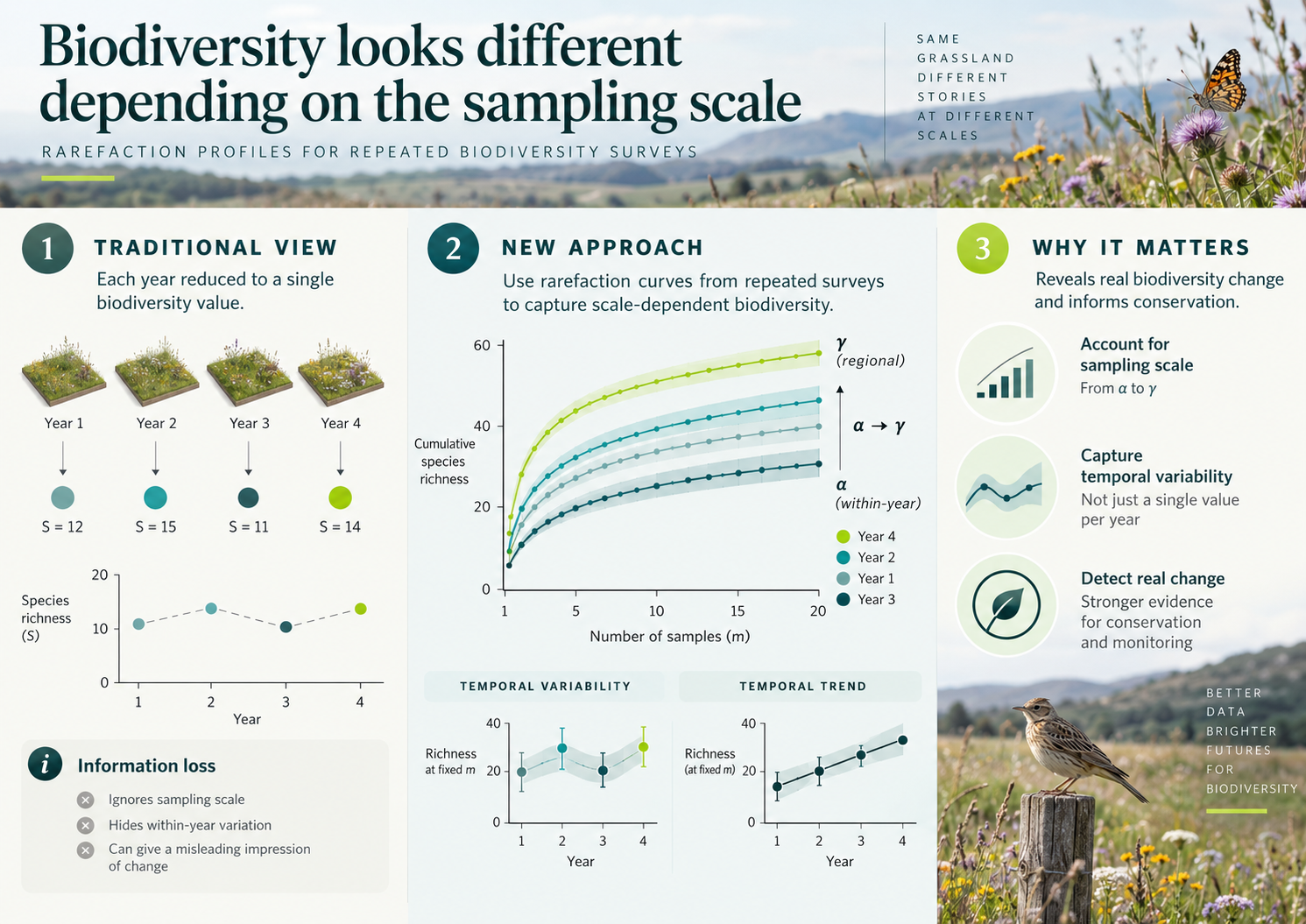
Biodiversity change is scale dependent. A temporal signal seen in individual plots does not necessarily persist when plots are pooled, and a cumulative change may emerge even when average plot-level diversity looks comparatively stable.
Repeated monitoring is nevertheless often summarised by one richness, diversity or composition value for each survey date. That endpoint can be informative, but it cannot show whether change is concentrated near the expected alpha-diversity scale, near the sampled-gamma endpoint, or along the transition between the two.
In our new paper in Ecological Informatics, we introduce rarefaction profiles for repeated biodiversity surveys: an accumulation-explicit framework that compares complete sample-based rarefaction curves through time rather than reducing each survey to a single value.
The method
A rarefaction curve for every survey occasion.
For each survey date, comparable sampling units are progressively accumulated and the target metric is recalculated at every value of m. At m = 1, the curve represents the expected value for one sampling unit. At m = N, all sampling units are pooled and the endpoint represents sampled gamma diversity for the defined sampling focus.
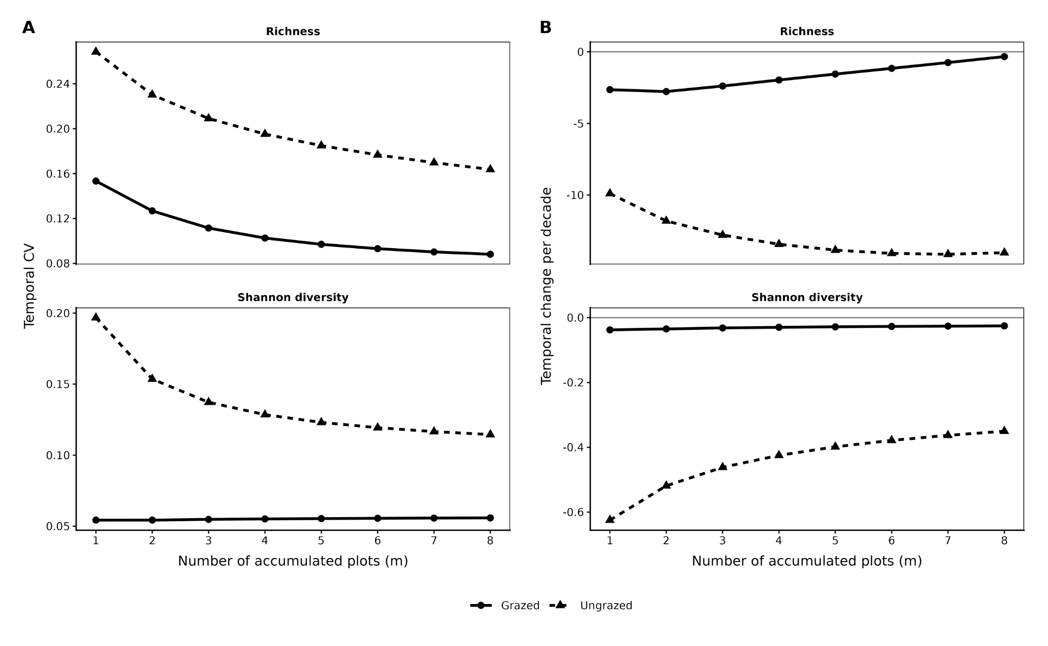
The annual curves are then compared at the same values of m. The method produces two complementary outputs: a temporal variability profile, describing how strongly the rarefied value varies among survey dates, and a temporal trend profile, describing the direction and magnitude of change through time.
The framework is metric-general. It can be applied to taxonomic diversity, functional diversity and directional community descriptors, provided the target quantity can be calculated after pooling subsets of sampling units.
The expected metric value for one sampling unit.
Sampling units are progressively pooled and the metric is recalculated.
The metric for the complete sampled community.
Worked example
Sixteen vegetation surveys between 2001 and 2019.
We illustrate the approach with the Monte Labbro long-term grassland experiment in southern Tuscany. Sixteen permanent plots were surveyed on 16 occasions between 2001 and 2019 and analysed as two balanced groups: eight grazed and eight ungrazed plots.
Species richness and Shannon diversity were used as the main taxonomic metrics. Functional richness quantified the occupied dominant-species trait space, while community-weighted mean (CWM) displacement measured movement in dominant trait composition relative to the first survey.
The empirical signal
Taxonomic and functional change did not tell the same story.
Taxonomic diversity showed the clearest treatment contrast. Ungrazed plots had higher temporal variability and stronger negative temporal change in both species richness and Shannon diversity than grazed plots. Resampling-based uncertainty supported these taxonomic contrasts across most or all of the accumulation gradient.
Functional responses differed. Point estimates indicated higher temporal variability of functional richness in grazed plots, while CWM displacement was more variable and increased more strongly in ungrazed plots. Sampling uncertainty around these functional treatment contrasts was substantially greater, so they are interpreted more cautiously.
The result is exactly why the full profile matters: the magnitude and support of biodiversity change can vary continuously between local and cumulative endpoints.
Why it matters
Monitoring should ask not only whether biodiversity changes, but where the change becomes visible.
The framework is diagnostic rather than mechanistic. A declining temporal-variability profile, for example, can be compatible with compensatory or asynchronous dynamics among sampling units, but the profile alone does not prove that mechanism. Independent ecological, compositional or spatial evidence is still needed.
Likewise, the accumulation index m is not automatically a spatial grain or extent. It is the number of sampling units pooled. This distinction keeps the method faithful to sample-based rarefaction while allowing temporal change to be interpreted explicitly between expected alpha diversity and sampled gamma diversity.
The approach therefore complements rather than replaces temporal beta-diversity analysis, time-series modelling, occupancy models and compositional analyses. Its contribution is to retain information that disappears when repeated surveys are compressed to one annual endpoint.
Open and reproducible
Data, code and a reusable R workflow.
The paper provides a reproducible implementation that returns survey-specific rarefaction curves, temporal variability and trend profiles, alpha and sampled-gamma summaries, whole-profile summaries and group contrasts. The stand-alone temporal_rarefy() development function is intended to support future integration into the Rarefy framework.